📈 TMA4135 - Mathematics 4D - Differential equations and Fourier analysis

Links

• NTNU
• Wikipendium (4D), (4N), (4K)
• Wiki Math, Q&A
• Exam Formula Sheet

Literature (PDFs)

• Preliminaries
• Numerical differentiation and numerical solution of boundary value problems
• Interpolation
• Numerical integration
• Rounding errors in numerical differentiation
• Partial derivatives
• Numerical Solution of Nonlinear Equations
• Complex Fourier Series
• Discrete Fourier Transform
• Numerical Solution of Partial Differential Equations
• Numerical Solution of Ordinary Differential Equations
• Numerical Solution of Ordinary Differential Equations, Part 2
• Summary

Laplace Transforms

The Laplace transform $F(s)$ of $f(t)$ is given by

$$F(s) = \mathscr{L}(f) = \int_0^\infty e^{-st}f(t) dt$$

The inverse transform is denoted

$$f(t) = \mathscr{L}^{-1}(F)$$

The Laplace transform is a linear operation.

Solving an ODE with Laplace Transform

The process of solving an ODE using the Laplace transform method consists of three steps:

1. The ODE is transformed into the subsidiary equation
2. The subsidiary equation is solved by purely algebraic manipulations.
3. The solution in Step 2 is transformed back, resulting in the solution of the given problem.

First Shifting Theorem, $s$-Shifting

$$\mathscr{L} \left\{ e^{at}f(t) \right\} = F(s-a)$$

Second Shifting Theorem, $t$-Shifting

$$\mathscr{L} \left\{ f(t-a)u(t-a) \right\} = e^{-as}F(s)$$

Existence and Uniqueness of Laplace Transforms

A function has a Laplace transform if it does not grow too fast, say, if for all $t \geq 0$ and some constants $M$ and $k$ it satisfies the growth restriction

$$|f(t)| \leq Me^{kt}$$

$f(t)$ must also be piecewise continous.

Laplace Transform of the Derivative and Integral

$$\mathscr{L}(f^{(n)}) = s^n F(s) - s^{n-1}f(0) - s^{n-2}f'(0) - \dots - f^{(n-1)}(0)$$

$$\mathscr{L}\left\{ \int_0^t f(\tau) d\tau \right\} = \frac{1}{s} F(s)$$

Dirac’s Delta Function

$$\delta(t-a) = \begin{cases} \infty, & \text{if } t = a\\ 0, & \text{otherwise} \end{cases}$$

$$\int_0^\infty \delta(t-a) dt = 1$$

The Sifting Property

$$\int_0^\infty g(t) \delta(t-a) dt = g(a)$$

The Laplace Transform and Convolution

If $f(t)$ and $g(t)$ are defined only on $t>0$

$$(f \ast g)(t) = \int_0^t f(\tau)g(t-\tau) d\tau$$

$$\mathscr{L} \left\{ f \ast g \right\} = \mathscr{L}(f) \cdot \mathscr{L}(g)$$

$$\int_0^t f(\tau) d\tau = 1 \ast f(t)$$

Convolution is commutative, distributive and associative.

Fourier Analysis

Fourier Series

Periodic Functions

A function $f(x)$ is called periodic if there is some positive number $p$, called a period of $f(x)$, such that

$$f(x + p) = f(x)$$

The Fourier Series and Coefficients

$$f(x) = a_0 + \sum_{n=1}^{\infty} \left(a_n \cos\left(\frac{n\pi}{L}x\right) + b_n \sin\left(\frac{n\pi}{L}x\right)\right)$$

For a periodic function $f(x)$ with period $p = 2L$ we have the Euler formulas

$$\begin{aligned} a_0 &= \frac{1}{2L} \int_{-L}^L f(x) dx \\ a_n &= \frac{1}{L} \int_{-L}^L f(x) \cos\left(\frac{n\pi}{L}x\right) dx \\ b_n &= \frac{1}{L} \int_{-L}^L f(x) \sin\left(\frac{n\pi}{L}x\right) dx \\ \end{aligned}$$

Even and Odd Functions

If $f(x)$ is an even function, that is, $f(-x) = f(x)$, then $b_n = 0$, reducing its Fourier series to a Fourier cosine series with

$$\begin{aligned} a_0 &= \frac{1}{L} \int_0^L f(x) dx \\ a_n &= \frac{2}{L} \int_0^L f(x) \cos\left(\frac{n\pi}{L}x\right) dx \\ \end{aligned}$$

If $f(x)$ is an odd function, that is, $f(-x) = -f(x)$, then $a_n = 0$, reducing its Fourier serier to a Fourier sine series with

$$\begin{aligned} b_n &= \frac{2}{L} \int_0^L f(x) \sin\left(\frac{n\pi}{L}x\right) dx \\ \end{aligned}$$

The Complex Fourier Series

$$f(x) = \sum_{n=-\infty}^\infty c_n e^{\frac{in\pi}{L} x}$$

where

$$c_n = \frac{1}{2L} \int_{-L}^L f(x) e^{-\frac{in\pi}{L} x} dx$$

For even functions $f$, the complex Fourier coefficients are real. For odd functions $f$, the complex Fourier coefficients are purely imaginary.

Euler's formula

The above is derived from the Euler's formula:

$$e^{ix} = \cos(x) + i \sin(x)$$

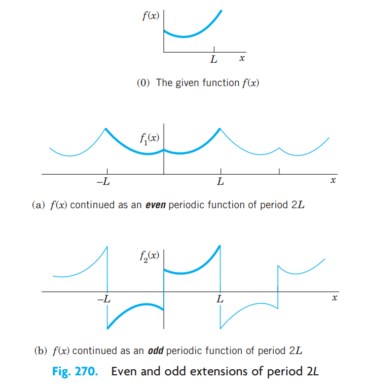
Half-Range Expansions

Approximation by Trigonometric Polynomials

The Nth partial sum of the Fourier series is an approximation of the given $f(x)$. The square error of the Nth partial sum is minimal only if the coefficients are the Fourier coefficients of $f$.

$$f(x) \approx a_0 + \sum_{n=1}^{N} \left(a_n \cos\left(\frac{n\pi}{L}x\right) + b_n \sin\left(\frac{n\pi}{L}x\right)\right)$$

Parseval’s Identity

$$2a_0^2 + \sum_{n=1}^\infty (a_n^2 + b_2^2) = \frac{1}{\pi} \int_{-\pi}^\pi f(x)^2 dx$$

The error of the Nth partial sum is equal to the difference of the left and right parts of Parseval's identity.

Fourier Integral

$$f(x) = \int_0^\infty \left[ A(w) \cos(wx) + B(w) \sin(wx) \right] dw$$

where

$$\begin{aligned} A(w) &= \frac{1}{\pi} \int_{-\infty}^\infty f(v) \cos(wv) dv \\ B(w) &= \frac{1}{\pi} \int_{-\infty}^\infty f(v) \sin(wv) dv \\ \end{aligned}$$

Fourier Transform

Fourier Transform and Its Inverse

The Fourier transform of $f$ is given by

$$\hat{f}(w) = \mathscr{F}(f) = \frac{1}{\sqrt{2\pi}} \int_{-\infty}^\infty f(x)e^{-iwx} dx$$

and the inverse Fourier transform is given by

$$f(x) = \mathscr{F}^{-1}(\hat{f}) = \frac{1}{\sqrt{2\pi}} \int_{-\infty}^\infty \hat{f}(w)e^{iwx} dw$$

Like the Laplace transform, the Fourier transform is a linear operation.

Fourier Transform of the Derivative and Integral

$$\mathscr{F} \left\{ f'(x) \right\} = iw \mathscr{F} \left\{ f(x) \right\}$$

$$\hat{f}'(w) = \mathscr{F} \left\{ -ixf(x) \right\}$$

The Fourier Transform and Convolution

$$\mathscr{F}(f \ast g) = \sqrt{2\pi} \mathscr{F}(f) \mathscr{F}(g)$$

$$(f \ast g)(x) = \int_{-\infty}^{\infty} \hat{f}(w)\hat{g}(w)e^{iwx} dw$$

Discrete Fourier Transform (DFT)

The discrete Fourier transform (DFT) $\bold{\hat{f}}$ of a signal $\bold{f}$ is given by

$$\bold{\hat{f}}_n = \sum_{k=0}^{N-1} \bold{f}_k e^{-i\frac{2\pi nk}{N}}$$

Alternatively, as a matrix-vector product:

$$\bold{\hat{f}} = \bold{F}_N \bold{f}$$

where $\bold{f}$ are sample values of $f(x)$,

$$w = w_N = e^{-2\pi i/N}$$

and

$$\bold{F}_N = \begin{bmatrix} w^0 & w^0 & w^0 & \dots & w^0 \\ w^0 & w^1 & w^2 & \dots & w^{N-1} \\ w^0 & w^2 & w^4 & \dots & w^{2(N-1)} \\ \vdots & \vdots & \vdots & \ddots & \vdots \\ w^0 & w^{N-1} & w^{2(N-1)} & \dots & w^{(N-1)^2} \\ \end{bmatrix}$$

The inverse transform is given by

$$\bold{f} = \bold{F}_N^{-1} \bold{\hat{f}} = \frac{1}{N}\overline{\bold{F}}_N \bold{\hat{f}}$$

DFT of Cosine and Sine

$$f_k = \cos\left( \frac{2\pi kn}{N} \right) \implies \hat{\bold{f}} = \left( 0_0, \dots, 0_{n-1}, \frac{N}{2}, 0, \dots, 0, \frac{N}{2}, 0_{N-n+1}, \dots, 0_{N-1}\right)$$

$$g_k = \sin\left( \frac{2\pi kn}{N} \right) \implies \hat{\bold{g}} = \left( 0_0, \dots, 0_{n-1}, -i\frac{N}{2}, 0, \dots, 0, +i\frac{N}{2}, 0_{N-n+1}, \dots, 0_{N-1}\right)$$

Partial Differential Equations (PDEs)

A PDE is an equation that contains one or more partial derivatives of an unknown function that depends on at least two variables.

ODE and PDE terminology

Basic Concepts of PDEs

Solution by Separating Variables. Use of Fourier Series

// TODO: Combine separation of variables explanation from wave and heat equations (difficult)

d'Alembert

A quick solution of the wave equation with initial conditions $u(x, 0) = f(x)$ and $u_t(x, 0) = g(x)$.

$$u(x, t) = \frac{1}{2} \left[f(x+ct) + f(x-ct)\right] + \frac{1}{2c} \int_{x-ct}^{x+ct} g(s) ds$$

Otherwise, we consider the following general solution with speed $c$ and manipulate to match the initial and boundary conditions

$$u(x, t) = \phi(x + ct) + \psi(x - ct)$$

Heat Equation: Modeling Very Long Bars. Solution by Fourier Integrals and Transforms

// TODO: Use of Fourier Transforms (difficult) // Solve PDE by Fourier transform

Rounding errors in numerical differentiation (4N)

Partial derivatives (4D)

Chain rule

For a scalar function $h(x) = f(g(x))$

$$\frac{\partial h}{\partial x} = \frac{\partial f}{\partial x}(g(x)) \cdot \frac{\partial g}{\partial x}(x)$$

For a vector function $g(t) = f(\overrightarrow{x}(t))$

$$\frac{\partial g}{\partial t} = \overrightarrow{\nabla} f(\overrightarrow{x}(t)) \cdot \frac{\partial \overrightarrow{x}}{\partial t}$$

where $\cdot$ is the dot product.

Gradient

The gradient of $f = f(x_1, x_2, \dots, x_n)$ is given by

$$\overrightarrow{\nabla} f = \left( \frac{\partial f}{\partial x_1}, \frac{\partial f}{\partial x_2}, \dots, \frac{\partial f}{\partial x_n} \right)$$

Directional derivative

The directional derivate of $f$, in the direction $\overrightarrow{u}$, is given by

$$D_{\overrightarrow{u}} f(\overrightarrow{a}) = \overrightarrow{\nabla} f(\overrightarrow{a}) \cdot \overrightarrow{u}$$

Jacobi matrix (Jacobian)

The Jacobian of $f = (f_1(x_1, \dots, x_n), \dots, f_n(x_1, \dots, x_n))$ is a matrix where each element is given by

$$J_{ij}(x) = \frac{\partial f_i}{\partial x_j}$$

For example, if $f = (f(x, y), g(x, y))$

$$J(\overrightarrow{x}) = \begin{bmatrix} \frac{\partial f}{\partial x} & \frac{\partial f}{\partial y} \\ \frac{\partial g}{\partial x} & \frac{\partial g}{\partial y} \\ \end{bmatrix}$$

Hess matrix (Hessian)

The Hessian of $f$, $H_f$ is the Jacobian of the gradient of $f$.

Partial Derivatives and Taylor Series

$$f(\overrightarrow{a} + \overrightarrow{h}) = f(\overrightarrow{a}) + \overrightarrow{\nabla} f(\overrightarrow{a}) \cdot \overrightarrow{h} + \overrightarrow{h}^T \cdot H_f(\overrightarrow{a}) \cdot \overrightarrow{h} + \dots$$

Preliminaries

Terminology

Order of convergence

The order of convergence is $p$ if there exists a positive constant $M$ such that

$$e_{k+1} \leq Me_k^p$$

where $e_k$ is the error of the $k$-th iteration.

The order can be numerically verified with the following approximation

$$p \approx \frac{\log(e_{k+2} / e_{k+1})}{\log(e_{k+1} / e_{k})}$$

$h$-dependent approximations

$e(h) = ||X-X(h)||$. The order of the approximation is $p$ if there exists a positive constant $M$ such that that

$$e(h) \leq Mh^p$$

alternatively, with Big $O$-notation

$$e(h) = O(h^p)$$

The order of $h$-dependent approximations can be numerically verified with the following approximation, where $h_{k+1}$ is some step size smaller then $h_k$.

$$p \approx \frac{\log(e(h_{k+1}) / e(h_k))}{\log(h_{k+1} / h_{k})}$$

Taylor Expansions

Given a function $f \in C^\infty[a, b]$, the Taylor polynomial of degree $m$ of $f$ around $a$ is then given by

$$f(x) = \sum_{k=0}^m \frac{(x - a)^k}{k!} f^{(k)}(a) + R_{m+1}(x)$$

Choose a point $x$ and an increment $h$ such that $x, x + h \in [a, b]$. The Taylor polynomial of degree $m$ of $f$ around $x$ is then given by

$$f(x + h) = \sum_{k=0}^m \frac{h^k}{k!} f^{(k)}(x) + R_{m+1}(x)$$

where

$$R_{m+1}(x) = \frac{h^{m+1}}{(m+1)!} f^{(m+1)}(\xi) = O(h^{m+1})$$

Intermediate Value Theorem

Let $f \in C[a, b]$ and let $x$ be some number between $f(a)$ and $f(b)$, then there exist at least one $\xi \in (a, b)$ such that $f(\xi) = x$.

Mean Value Theorem

Let $f \in C^1[a, b]$. Then there exists at least one $\xi \in (a, b)$ such that

$$f'(\xi) = \frac{f(b) - f(a)}{b - a}$$

Mean Value Theorem for Integrals

Let $f \in C[a, b]$ and $g$ an integrable function that does not change sign on $[a, b]$. Then there exists at least one $\xi \in (a, b)$ such that

$$\int_a^b f(x)g(x)dx = f(\xi) \int_a^b g(x) dx$$

Numerical Differentiation and Numerical Solution of Boundary Value Problems

Constructing a finite difference scheme for solving a linear BVP is composed from the following steps:

1. Discretize the domain on which the equation is defined.
2. On each grid point, replace the derivatives with an approximation, using the values in neighbouring grid points.
3. Replace the exact solutions by its approximations.
4. Solve the resulting system of equations with boundary and or intial conditions.

Numerical differentiation

$$f'(x) = \begin{cases} \frac{f(x+h)-f(x)}{h} - \frac{h}{2}f''(\xi), & \text{Forward difference} \\ \frac{f(x)-f(x-h)}{h} + \frac{h}{2}f''(\xi), & \text{Backward difference} \\ \frac{f(x+h)-f(x-h)}{2h} - \frac{h^2}{6}f'''(\xi), & \text{Central difference} \\ \end{cases}$$

$$f''(x) = \frac{f(x+h)-2f(x)+f(x-h)}{h^2} - \frac{h^2}{12}f^{(4)}(\xi) \quad \text{Central difference}$$

When approximating, we use only the first terms. The second terms then become the error. The errors may also be written as $O(h)$ for forward and backward difference and $O(h^2)$ for central difference for the first and second derivative.

Interpolation

With the direct polynomial approach to solving an interpolation problem where $n+1$ points $(x_i, y_i)$ are given, we let $p(x) = c_nx^n + c_{n-1}x^{n-1} + \dots + c_1x_1 + c_0$ and create a linear system of $n + 1$ equations $p(x_i) = y_i$, which we solve for all $c_i$.

With spline interpolation, we use piecewise polynomials. Linear splines results in straight lines between each point. Cubic splines are the most important in practise.

Numerical integration

A numerical quadrature or a quadrature rule is a formula, usually of the form of the left, for approximating integrals such as the one on the right. We call $w_i$ weights and $x_i$ nodes.

$$Q[f](a, b) = \sum_{i=0}^n w_i f(x_i) \approx I[f](a, b) = \int_a^b f(x) dx$$

In practice, we will not use a single (or simple) quadrature for the whole interval $[a, b]$, but rather apply a quadrature on each of $m$ subintervals $[X_j , X_{j+1}], j = 0, 1, \dots, m-1$, and then add the results together. This leads to composite quadratures yielding the approximation

$$I[f](a, b) \approx \sum_{j=0}^{m-1} Q[f] (X_j, X_{j+1})$$

It is common to define a quadrature from nodes on the standard interval $[-1, 1]$, and then transferring it to an arbitrary interval $[a, b]$. This transformation is done by

$$x = \frac{b-a}{2}t + \frac{b+a}{2}, \qquad dx = \frac{b-a}{2}dt$$

See the Simpson's rule below for an example.

Quadrature Rule Examples

Simpson's Rule

$$S(-1, 1) = \frac{1}{3}\left[ f(-1) + 4f(0) + f(1) \right]$$

$$S(a, b) = \frac{b-a}{6}\left[ f(a) + 4f\left(\frac{a+b}{2}\right) + f(b)\right]$$

$$S_m(a, b) = \frac{h}{3} \left[ f(x_0) + 4\sum_{j=0}^{m-1} f(x_{2j+1}) + 2\sum_{j=1}^{m-1}f(x_{2j}) + f(x_{2m}) \right]$$

$$E_{S}(a, b) = I[f](a, b) - S(a, b) = - \frac{(b-a)^5}{2880} f^{(4)}(\xi)$$

$$E_{S_m}(a, b) = I[f](a, b) - S_m(a, b) = - \frac{(b-a)h^4}{180} f^{(4)}(\xi)$$

Trapezoidal rule

$$T(a, b) = \frac{b-a}{2}(f(a) + f(b))$$

$$T_m(a, b) = h \left[ \frac{1}{2} f(x_0) + \sum_{j=1}^{m-1} f(x_j) + \frac{1}{2} f(x_m) \right]$$

$$E_{T}(a, b) = I[f](a, b) - T(a, b) = - \frac{(b-a)^3}{12} f''(\xi)$$

$$E_{T_m}(a, b) = I[f](a, b) - T_m(a, b) = - \frac{(b-a)h^2}{12} f''(\xi)$$

The Midpoint Rule

$$M(a, b) = (b-a) f \left( \frac{a + b}{2} \right)$$

$$M_m(a, b) = \frac{b-a}{m} \sum_{j=0}^{m-1} f(x_{j+1/2})$$

$$E_{M}(a, b) = I[f](a, b) - M(a, b) = - \frac{(b-a)^3}{24} f''(\xi)$$

$$E_{M_m}(a, b) = I[f](a, b) - M_m(a, b) = - \frac{(b-a)h^2}{24} f''(\xi)$$

Gauss-Legendre Quadrature

For the standard interval $[−1, 1]$ choose the nodes as the zeros of the polynomial of degree $n$:

$$L_n(t) = \frac{d^n}{dt^n} (t^2-1)^n$$

The resulting quadrature rules have a degree of precision $d = 2n − 1$, and the corresponding composite rules have a convergence order of $2n$.

Error Estimation for Quadratures

We can create an upper bound for the error by maximizing the $f^{(n)}(\xi)$ term. This bound, however, often vastly overestimates the actual error.

A better error estimation may be found by:

• Write $E_m$ as $C_mh^n$ where $n$ is given by the exponent of $h$ in $E_m$
• Write $E_{2m}$ as $C_{2m}\left(\frac{h}{2}\right)^n$
• Let $C = C_m = C_{2m}$
• Solve $I - Q_m \approx Ch^n; \quad I - Q_{2m} \approx C\left(\frac{h}{2}\right)^n;$ for $I$
• Insert this $I$ into $E_{2m} = I - Q_{2m}$ for an estimate of $E_{2m}$

Adaptive Integration

An adaptive quadrature is a recursive algorithm which for each step accepts the result $Q(a,b) + \Epsilon(a,b)$ if $|\Epsilon(a, b)| \leq \text{Tol}$, otherwise it splits the interval in two halves and calls the procedure on these subintervals with tolerance $\text{Tol}/2$.

Numerical Solution of Nonlinear Equations

Existence and uniqueness of a solution

The intermediate value theorem is used to prove the existence of a solution, and monotonicity ($|f'(x)| > 0$) proves that the solution is unique.

Fixed Point Iterations

Given $g$ such that $r = g(r)$, and a starting value $x_0$

$$x_{k+1} = g(x_k), \qquad k = 0, 1, 2, \dots$$

If $g$ is continous and $a < g(x) < b$ on $[a, b]$ and there exist a positive constant $L$ such that $|g'(x)| \leq L < 1$ for all $x \in [a, b]$ then

• $g$ has a unique fixed point $r$ in (a, b)
• The fixed point iterations converges toward $r$ for $x_0 \in [a, b]$
• The error $e_{k+1} = r - x_{k+1}$ satisfies:
  • $|e_{k+1}| \leq L|e_k|$, error reduction rate
  • $|e_{k+1}| \leq \frac{L^{k+1}}{1-L}|x_1-x_0|$, a-priori error estimate
  • $|e_{k+1}| \leq \frac{L}{1-L}|x_{k+1}-x_k|$, a-posteriori error estimate

Newton's Method

Given $f(x) = 0$ and a starting value $x_0$, Newton's method is given by

$$x_{k+1} = x_k - \frac{f(x_k)}{f'(x_k)}, \qquad k = 0, 1, 2, \dots$$

Assume that $f$ has a root $r$, and is two times continuously differentiable on $I_\delta = [r - \delta, r + \delta]$ for some $\delta > 0$. If there is a positive constant $M$ such that

$$\left| \frac{f''(x_1)}{f'(x_2)} \right| \leq 2M, \qquad \text{ for all } x_1, x_2, \in I_\delta$$

then Newton's iterations converge quadratically,

$$|e_{k+1}| \leq M|e_k|^2$$

for all starting values $x_0$ satisfying $|x_0 - r| \leq \min\{1/M, \delta\}$.

Newton's Method for Systems of Equations

Given a vector function $\bold{f(x)}: \mathbb{R}^m \rightarrow \mathbb{R}^m$, its Jacobian $J(\bold{x})$ and a starting value $\bold{x}_0$. For $k = 0, 1, 2, \dots$

• Solve the system $J(\bold{x}_k) \Delta_k = -\bold{f}(\bold{x}_k)$
• Let $\bold{x}_{k+1} = \bold{x}_k + \Delta_k$

Alternatively, with the inverse Jacobian $J(\bold{x})^{-1}$

• $\bold{x}_{k+1} = \bold{x}_k - J(\bold{x_k})^{-1}\bold{f}(\bold{x}_k)$

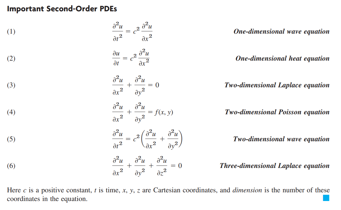
Numerical Solution of Partial Differential Equations

Explicit Scheme

For an explicit scheme, we follow the same procedure as in Numerical Solutions of BVP, but use the notation $U_i^n \approx u(x_i, t_n)$ since we now have two variables.

For values outside of the domain (e.g. $U_{i}^{-i}$ or $U_{i}^{n+1}$), we once again use an approximation (e.g. central difference) to represent the value from values within the domain.

The Explicit Euler method uses central differences in the $x$-direction, and forward differences in the $t$-direction.

Wave Equation

The Courant–Friedrichs–Lewy (CFL) stability condition states that our numerical method is stable for the wave equation if and only if

$$c\frac{k}{h} \leq 1$$

Heat Equation

Our numerical method is once again stable for the heat equation if and only if

$$c^2 \frac{h}{k^2} \leq \frac{1}{2}$$

Implicit Scheme (Implicit Euler)

By swapping the forward differences in $t$-direction of the explicit Euler method with backward differences, we get the implicit Euler method. The result is a system of linear equations. The implicit Euler method for the heat equation is unconditionally stable.

Crank-Nicolsen method

The idea of the Crank-Nicolson method is to combine the updates for the explicit and the implicit Euler methods.

// TODO: Crank-Nicolsen method

Numerical Solution of Ordinary Differential Equations

Scalar ODE

A scalar ODE is an equation of the form

$$y'(t) = f(t, y(t)), \qquad y(t_0) = y_0$$

The initial condition is required for a unique solution, and makes it an initial value problem (IVP).

For example,

$$y' = -2ty$$

has the solution

$$y(t) = Ce^{-t^2}$$

where C depends on the initial condition $y(t_0)$.

System of ODEs

A system of ODEs (in vector form) is given by

$$\bold{y}'(t) = \bold{f}(t, \bold{y}(t)), \qquad \bold{y}(t_0) = \bold{y}_0$$

Higher order ODEs

An ODEs of order $m$

$$y^{(m)} = f(t, y, y', \dots, y^{(m-1)}), \quad y(t_0) = y_0, \dots$$

may be written as a system of first order ODEs like the following

$$\bold{z} = \begin{bmatrix} y \\ y' \\ \vdots \\ y^{(m-1)} \end{bmatrix}, \qquad \bold{z'} = \begin{bmatrix} y' \\ y'' \\ \vdots \\ f(t, y, y', \dots, y^{(m-1)}) \end{bmatrix}, \qquad \bold{z}_0 = \begin{bmatrix} y_0 \\ y'_0 \\ \vdots \\ y_0^{(m-1)} \end{bmatrix}$$

Euler's method

$$\bold{y}_{n+1} = \bold{y}_n + h\bold{f}(t_n, \bold{y}_n)$$

Heun's method

$$\begin{aligned} \bold{k}_1 &= \bold{f}(t_n, \bold{y}_n), \\ \bold{k}_2 &= \bold{f}(t_n + h, \bold{y}_n + h\bold{k}_1), \\ \bold{y}_{n+1} &= \bold{y}_n + \frac{h}{2}(\bold{k}_1 + \bold{k}_2), \\ \end{aligned}$$

Runge–Kutta methods

An $s$-stage Runge-Kutta method is given by

$$\begin{aligned} \bold{k}_i &= \bold{f}(t_n + c_ih, \bold{y}_n + h \sum_{j=1}^s a_{ij}\bold{k_j}), \qquad i = 1,2,\dots,s, \\ \bold{y}_{n+1} &= \bold{y}_n + h\sum_{i=1}^s b_i \bold{k}_i \end{aligned}$$

The method is defined by its coefficients $a_{ij}, b_i, c_i$, which may be visualized in a Butcer tableau. The method is explicit if $a_{ij} = 0$ whenever $i \geq j$; otherwise it is implicit.

Lipschitz Continuity

A function $f$ is lipschitz continous if there exists a constant $L$ such that

$$\| f(t, y_1) - f(t, y_2) \| \leq L \| y_1 - y_2 \| \qquad \text{for all $t, y_1, y_2$ in the domain}$$

Consider the IVP $\bold{y}' = \bold{f}(t, \bold{y}), \quad \bold{y}(t_0) = \bold{y}_0$. If $f(t, y)$ is lipschitz continous in $D$, then the ODE has one and only one solution in $D$.

Order of a method

A method is of order $p > 0$ if there is a constant $C > 0$ such that

$$\| \bold{e}_N \| = \|\bold{y}(t_{end}) - \bold{y}_N \| \leq Ch^p, \qquad \text{where} h = (t_{end} - t_0)/N$$

Order conditions for Runge–Kutta methods

See the formula sheet

Error Estimation for Numerical Solutions of ODEs

A reasonable approximation to the unknown local error $\bold{l}_{n+1}$ is the local error estimate $\bold{le}_{n+1}$

$$\bold{le}_{n+1} = \hat{\bold{y}}_{n+1} - \bold{y}_{n+1} \approx \bold{l}_{n+1}$$

where $\bold{y}_{n+1}$ is found by a method of order $p$ and $\hat{\bold{y}}_{n+1}$ is found by a method of order $p+1$.

Stepsize control

After a step $n$, the next step size is given by

$$h_{new} = P \left( \frac{\text{Tol}}{\| \bold{le}_{n+1} \|} \right)^{\frac{1}{p + 1}} h_n$$

where the pessimist factor $P < 1$ is some chosen constant, normally between $0.5$ and $0.95$. We only move forwards if $|\bold{le}_{n+1} < \text{Tol}$.

Runge–Kutta Methods with an Error Estimate

The error estimate is then given by

$$\bold{le}_{n+1} = h\sum_{i=1}^s (\hat{b}_i - b_i)\bold{k}_i$$

Linear stability analysis

Linear stability can be analyzed by studying the very simple linear test equation

$$y' = \lambda y, \qquad y(0) = y_0$$

One step of some Runge–Kutta method applied to the linear test equation can always be written as

$$y_{n+1} = R(z)y_n, \qquad z = \lambda h$$

where $R(z)$ is called the stability function of the method.

The stability region of a method is defined by

$$S = \{ z \in \mathbb{C} : |R(z)| \leq 1 \}$$

To get a stable numerical solution, we have to choose the step size $h$ such that $z = \lambda h \in S$.

$A$-stable methods

A method is $A$-stable if the stability region $S$ covers $\mathbb{C}^-$. This means that it is stable for all $\lambda \in \mathbb{C}^-$ independent of $h$. Explicit methods can never be $A$-stable.